Introduction to binaryPPIclassifier
Philipp Trepte
2024-01-12
introduction.RmdUsing machine learning (ML) algorithms to classify quantitative PPI results
This vignette gives an introduction to the
binaryPPIclassifier package. A support vector
machine learning or random forest algorithm in
combination with multi-adaptive sampling is trained on a data set
containing positive and random/negative reference protein-protein
interaction (PPI) results. The generated models are then applied to a
set of PPIs with unknown classification and their likelihood to be
positive or negative is predicted.
Installation
You can install the development version of binaryPPIclassifier from GitHub with:
# install.packages("devtools")
devtools::install_github("philipptrepte/binary-PPI-classifier")

library(binaryPPIclassifier)
Requirements
The input data should have been pre-processed or tidied if necessary.
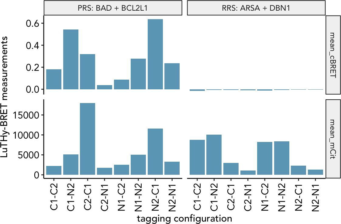
Example dataset: LuTHy results from PRS-v2 and RRS-v2
We used the LuTHy assay (Trepte et al. Mol Sys Biol 2018) to detect protein-protein interactions between 60 PRS-v2 and 78 RRS-v2 (Choi et al. Nat Com 2019), which were each tested in 8 tagging configutation with the LuTHy-BRET and LuTHy-LuC assay versions (Trepte & Secker et al. bioRxiv 2023).
The dataset contains in-cell LuTHy-BRET and cell-free LuTHy-LuC measurements. For the LuTHy-BRET we measure the Acceptor protein expression mean_mCit, which directly influences the BRET ratio mean_cBRET. For the LuTHy-LuC, we measure the raw luminescence value after precipitation mean_LumiOUT of the Donor protein which is normalized to its expression resulting in the mean_cLuC.
For more details on the LuTHy assay and its measurement parameters, please read:
Trepte, P. et al. LuTHy: a double-readout bioluminescence-based two-hybrid technology for quantitative mapping of protein–protein interactions in mammalian cells. Mol Syst Biol 14, e8071 (2018). [Link]
Trepte, P. & Secker, C. et al. AI-guided pipeline for protein-protein interaction drug discovery identifies a SARS-CoV-2 inhibitor. bioRxiv 2023.06.14.544560 (2023) doi:10.1101/2023.06.14.544560. [Link]
Loading of the data
data("luthy_reference_sets")| Donor | Donor_tag | Donor_protein | Acceptor | Acceptor_tag | Acceptor_protein | complex | interaction | sample | orientation | data | score |
|---|---|---|---|---|---|---|---|---|---|---|---|
| 5575 | N1 | BAD | 5168 | N2 | BCL2L1 | PRS | BAD + BCL2L1 | BAD+BCL2L1 | N1-N2 | mean_LumiOUT | 2.984230e+05 |
| 5575 | N1 | BAD | 5431 | C2 | BCL2L1 | PRS | BAD + BCL2L1 | BAD+BCL2L1 | N1-C2 | mean_LumiOUT | 6.519733e+04 |
| 5838 | C1 | BAD | 5168 | N2 | BCL2L1 | PRS | BAD + BCL2L1 | BAD+BCL2L1 | C1-N2 | mean_LumiOUT | 4.999130e+05 |
| 5838 | C1 | BAD | 5431 | C2 | BCL2L1 | PRS | BAD + BCL2L1 | BAD+BCL2L1 | C1-C2 | mean_LumiOUT | 7.323867e+04 |
| 5694 | N2 | BCL2L1 | 5049 | N1 | BAD | PRS | BAD + BCL2L1 | BCL2L1+BAD | N2-N1 | mean_LumiOUT | 4.725640e+05 |
| 5957 | C2 | BCL2L1 | 5049 | N1 | BAD | PRS | BAD + BCL2L1 | BCL2L1+BAD | C2-N1 | mean_LumiOUT | 3.265000e+04 |
| 5694 | N2 | BCL2L1 | 5312 | C1 | BAD | PRS | BAD + BCL2L1 | BCL2L1+BAD | N2-C1 | mean_LumiOUT | 2.395853e+06 |
| 5957 | C2 | BCL2L1 | 5312 | C1 | BAD | PRS | BAD + BCL2L1 | BCL2L1+BAD | C2-C1 | mean_LumiOUT | 9.105850e+04 |
| 5575 | N1 | BAD | 5168 | N2 | BCL2L1 | PRS | BAD + BCL2L1 | BAD+BCL2L1 | N1-N2 | mean_mCit | 5.011334e+03 |
| 5575 | N1 | BAD | 5431 | C2 | BCL2L1 | PRS | BAD + BCL2L1 | BAD+BCL2L1 | N1-C2 | mean_mCit | 2.547251e+03 |
| 5838 | C1 | BAD | 5168 | N2 | BCL2L1 | PRS | BAD + BCL2L1 | BAD+BCL2L1 | C1-N2 | mean_mCit | 5.091001e+03 |
| 5838 | C1 | BAD | 5431 | C2 | BCL2L1 | PRS | BAD + BCL2L1 | BAD+BCL2L1 | C1-C2 | mean_mCit | 2.249626e+03 |
| 5694 | N2 | BCL2L1 | 5049 | N1 | BAD | PRS | BAD + BCL2L1 | BCL2L1+BAD | N2-N1 | mean_mCit | 3.293543e+03 |
| 5957 | C2 | BCL2L1 | 5049 | N1 | BAD | PRS | BAD + BCL2L1 | BCL2L1+BAD | C2-N1 | mean_mCit | 1.744793e+03 |
| 5694 | N2 | BCL2L1 | 5312 | C1 | BAD | PRS | BAD + BCL2L1 | BCL2L1+BAD | N2-C1 | mean_mCit | 1.157221e+04 |
| 5957 | C2 | BCL2L1 | 5312 | C1 | BAD | PRS | BAD + BCL2L1 | BCL2L1+BAD | C2-C1 | mean_mCit | 1.801200e+04 |
| 5575 | N1 | BAD | 5168 | N2 | BCL2L1 | PRS | BAD + BCL2L1 | BAD+BCL2L1 | N1-N2 | mean_cBRET | 2.765355e-01 |
| 5575 | N1 | BAD | 5431 | C2 | BCL2L1 | PRS | BAD + BCL2L1 | BAD+BCL2L1 | N1-C2 | mean_cBRET | 8.709540e-02 |
| 5838 | C1 | BAD | 5168 | N2 | BCL2L1 | PRS | BAD + BCL2L1 | BAD+BCL2L1 | C1-N2 | mean_cBRET | 5.438252e-01 |
| 5838 | C1 | BAD | 5431 | C2 | BCL2L1 | PRS | BAD + BCL2L1 | BAD+BCL2L1 | C1-C2 | mean_cBRET | 1.808837e-01 |
| 5694 | N2 | BCL2L1 | 5049 | N1 | BAD | PRS | BAD + BCL2L1 | BCL2L1+BAD | N2-N1 | mean_cBRET | 2.366357e-01 |
| 5957 | C2 | BCL2L1 | 5049 | N1 | BAD | PRS | BAD + BCL2L1 | BCL2L1+BAD | C2-N1 | mean_cBRET | 3.644020e-02 |
| 5694 | N2 | BCL2L1 | 5312 | C1 | BAD | PRS | BAD + BCL2L1 | BCL2L1+BAD | N2-C1 | mean_cBRET | 6.381235e-01 |
| 5957 | C2 | BCL2L1 | 5312 | C1 | BAD | PRS | BAD + BCL2L1 | BCL2L1+BAD | C2-C1 | mean_cBRET | 3.185715e-01 |
| 5575 | N1 | BAD | 5168 | N2 | BCL2L1 | PRS | BAD + BCL2L1 | BAD+BCL2L1 | N1-N2 | mean_cLuC | 7.362038e-01 |
| 5575 | N1 | BAD | 5431 | C2 | BCL2L1 | PRS | BAD + BCL2L1 | BAD+BCL2L1 | N1-C2 | mean_cLuC | 6.521600e-01 |
| 5838 | C1 | BAD | 5168 | N2 | BCL2L1 | PRS | BAD + BCL2L1 | BAD+BCL2L1 | C1-N2 | mean_cLuC | 1.001871e+00 |
| 5838 | C1 | BAD | 5431 | C2 | BCL2L1 | PRS | BAD + BCL2L1 | BAD+BCL2L1 | C1-C2 | mean_cLuC | 7.442408e-01 |
| 5694 | N2 | BCL2L1 | 5049 | N1 | BAD | PRS | BAD + BCL2L1 | BCL2L1+BAD | N2-N1 | mean_cLuC | 1.196843e+00 |
| 5957 | C2 | BCL2L1 | 5049 | N1 | BAD | PRS | BAD + BCL2L1 | BCL2L1+BAD | C2-N1 | mean_cLuC | 5.047924e-01 |
| 5694 | N2 | BCL2L1 | 5312 | C1 | BAD | PRS | BAD + BCL2L1 | BCL2L1+BAD | N2-C1 | mean_cLuC | 2.608016e+00 |
| 5957 | C2 | BCL2L1 | 5312 | C1 | BAD | PRS | BAD + BCL2L1 | BCL2L1+BAD | C2-C1 | mean_cLuC | 1.114725e-01 |
| Column name | Description |
|---|---|
| Donor | unique id to identify the donor construct |
| Donor_tag | indicates if the donor protein is tagged N-terminally (“N”) or C-terminally (“C”) |
| Donor_protein | a protein identifier, e.g. BCL2L1 |
| Acceptor | unique id to identify the acceptor construct |
| Acceptor_tag | indicates if the acceptor protein is tagged N-terminally (“N”) or C-terminally (“C”) |
| Acceptor_protein | a protein identifier, e.g. BAD |
| complex | should contain information if it is a reference interaction (e.g. “PRS”/“RRS”) or if it is part of any other known complex (e.g. “LAMTOR”) |
| interaction | should indicate the tested interaction independent on the tagging configuration, e.g. “BAD + BCL2L1” |
| sample | should indicate the tested interaction dependent on the tagging configuration, e.g. “BCL2L1 + BCL2L1” |
| orientation | indicates the exact tagging orientation of the first indicated donor protein (e.g. N1) and the second indicated acceptor protein (e.g. N2): N1-N2 for BAD + BCL2L1 and N2-N1 for BCL2L1 + BAD |
| data | indicates the type of data measured for an indicated interaction, e.g. “mean_cBRET” or “mean_cLuC” |
| score | The corresponding data value |
Example interaction: BAD + BCL2L1
Tagging configuration (orientation column) |
Example (NL = NanoLuc; mCit = mCitrine) | interaction | sample |
|---|---|---|---|
| C1-C2 | BAD-NL + BCL2L1-mCit | BAD + BCL2L1 | BAD + BCL2L1 |
| C1-N2 | BAD-NL + mCit-BCL2L1 | BAD + BCL2L1 | BAD + BCL2L1 |
| N1-C2 | NL-BAD + BCL2L1-mCit | BAD + BCL2L1 | BAD + BCL2L1 |
| N1-N2 | NL-BAD + mCit-BCL2L1 | BAD + BCL2L1 | BAD + BCL2L1 |
| C2-C1 | BCL2L1-NL + BAD-mCit | BAD + BCL2L1 | BCL2L1 + BAD |
| C2-N1 | BCL2L1-NL + mCit-BAD | BAD + BCL2L1 | BCL2L1 + BAD |
| N2-C1 | NL-BCL2L1 + BAD-mCit | BAD + BCL2L1 | BCL2L1 + BAD |
| N2-N1 | NL-BCL2L1 + mCit-BAD | BAD + BCL2L1 | BCL2L1 + BAD |
Usage
The ML algorithms for the LuTHy-BRET and LuTHy-LuC are trained on the mean_cBRET and mean_mCit or mean_cLuC and mean_LumiOUT features, respectively. Other assays that provide only one quantitative measurement, like the mN2H, can be trained only on this one feature. Training on more than two features is also possible but has not been tested.
| Assay | Training features (data column) |
|---|---|
| LuTHy-BRET | mean_cBRET, mean_mCit |
| LuTHy-LuC | mean_cLuC, mean_LumiOUT |
ppi.prediction()
The function ppi.prediction is used to predict the
classification probability of a PPIdf with unknown
classification labels by training an svm or
randomforest machine learning algorithm on a set of
reference interactions that contain classification labels. The
parameters to be specified for the function can be found in the
Documentation ?ppi.prediction.
In the following example, we use the luthy_reference_set
example data to compile distinct training sets by sampling 50 times
(ensembleSize = 50) from the entire
referenceSet dataset. Weighted sampling is performed
(sampling = “weighted”) using the mean_cBRET data
(weightBy = “mean_cBRET”) from all interactions
(cutoff = “all”). The data will not be further scaled
(method.scaling = “none”) and we specify that in the
complex column the negative/random interactions are indicated by “RRS”
(negative.reference = “RRS”). We further specify that as
training features for the LuTHy-BRET the mean_cBRET and mean_mCit
(assay = c(“mean_cBRET”, “mean_mCit”) will be used to train
the SVM algorithms (model.type = “svm”). For the SVM
algorithm a linear kernel will be used (kernelType =
“linear”) with a cost of constraints violation of 100 (C =
100). During training, the class labels of the reference set are
reclassified in 5 iterations (iter = 5)
example_ppi_prediction <- ppi.prediction(PPIdf = luthy_reference_sets,
               referenceSet = luthy_reference_sets,
               ensembleSize = 50,
               sampling = "weighted",
               weightBy = "mean_cBRET",
               cutoff = "all",
               method.scaling = "none",
               negative.reference = "RRS",
               assay = ("mean_cBRET", "mean_mCit"),
               model.type = "svm",
               kernelType = "linear",
               C = 100,
               iter = 5)
data("example_ppi_prediction")The resulting list contains the following objects:
| List object | Description |
|---|---|
| predTrainDf | Data frame of the training set containing the predicted classifier
probabilities in the column predTrainMat
|
| predDf | Data frame of the PPIdf test set containing the predicted classifier
probabilities in the column predMat
|
| predTrain.model.e | List for each ensembleSize as defined in
ppi.prediction() containing the trained ML models used to
predict the classification of the reference training set |
| training.sets | List for each ensembleSize as defined in
ppi.prediction() containing the training sets used to train
each ML model |
| negative.reference | as specified in ppi.prediction()
|
| model.type | as specified in ppi.prediction()
|
| model.e | List for each ensembleSize as defined in
ppi.prediction() containing the trained ML models used to
predict the classification of the PPIdf test set |
| testMat | Matrix of the PPIdf test set containing the features used for training |
| trainMat | Matrix of the reference training set containing the features used for training |
| label | Classifier labels of the reference training set interactions |
| cutoff | as specified in ppi.prediction()
|
| inclusion | as specified in ppi.prediction()
|
| ensembleSize | as specified in ppi.prediction()
|
| sampling | as specified in ppi.prediction()
|
| kernelType | as specified in ppi.prediction()
|
| iter | as specified in ppi.prediction()
|
| C | as specified in ppi.prediction()
|
| gamma | as specified in ppi.prediction()
|
| coef0 | as specified in ppi.prediction()
|
| degree | as specified in ppi.prediction()
|
| top | as specified in ppi.prediction()
|
| seed | as specified in ppi.prediction()
|
| system.time | System time when the function was run |
Plotting the results from the ML predictions
The package provides helper functions, to plot the results from the
ML predictions (@ref(fig:MLresultPlot)). probGrid.plot will
generate a probability grid, probDis.plot will show the
probability distribution against the first feature and a receiver
operating characteristic curve can be plotted using the
roc.plot function. Finally, the recovery rates at 50%, 75%
and 95% can be plotted using the function
recovery.plot.
cowplot::plot_grid(
    probGrid.plot(example_ppi_prediction, ylim = c(-0.1, 0.8)),
    probDis.plot(example_ppi_prediction),
    roc.plot(example_ppi_prediction),
    recovery.plot(example_ppi_prediction),
  ncol = 2, align = "hv", axis = "tlrb", labels = "AUTO"
)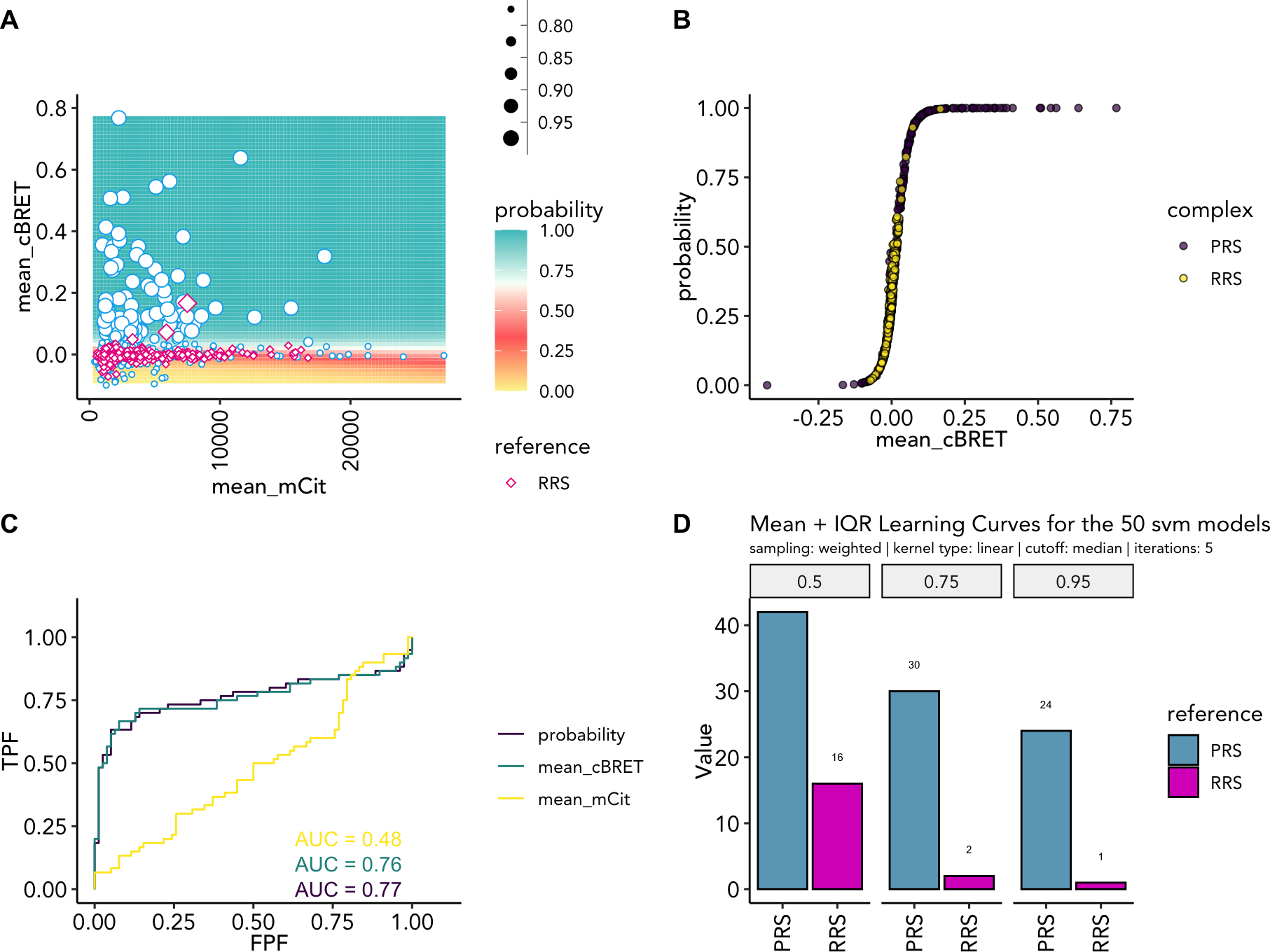
Training results as (A) probability grid; (B) probability distribtuoin; (C) ROC curve plotting the training features and the probability; (D) recovery rates at 50%, 75% and 95% probability
Confusion Matrix
To evaluate the performance of the classification model, we can
calculate the confusion matrix using the function
confusion.matrix which is based on the
caret::confusionMatrix function.
example_confusion_matrix <- confusion.matrix(example_ppi_prediction)A tabulated confusion matrix can be accessed by
example_confusion_matrix$confusionMatrixDf
| PRS | RRS | |
|---|---|---|
| PRS: 50% | 42 | 14 |
| RRS: 50% | 18 | 64 |
| PRS: 75% | 30 | 2 |
| RRS: 75% | 30 | 76 |
| PRS: 95% | 23 | 1 |
| RRS: 95% | 37 | 77 |
Detailed information and statistics can be assessed by
example_confusion_matrix$confusionMatrixList for at 50%,
75% and 95% probability.
#> Confusion Matrix and Statistics
#>
#>           Reference
#> Prediction PRS RRS
#>        PRS  23   1
#>        RRS  37  77
#>
#>                Accuracy : 0.7246
#>                  95% CI : (0.6422, 0.7972)
#>     No Information Rate : 0.5652
#>     P-Value [Acc > NIR] : 8.065e-05
#>
#>                   Kappa : 0.3981
#>
#>  Mcnemar's Test P-Value : 1.365e-08
#>
#>             Sensitivity : 0.3833
#>             Specificity : 0.9872
#>          Pos Pred Value : 0.9583
#>          Neg Pred Value : 0.6754
#>              Prevalence : 0.4348
#>          Detection Rate : 0.1667
#>    Detection Prevalence : 0.1739
#>       Balanced Accuracy : 0.6853
#>
#>        'Positive' Class : PRS
#> 
learning.curve()
To evaluate the model performance, we can plot learning curves using
the function learning.curve(). Performance metrics
(accuracy, hinge loss, binary cross-entropy loss) are plotted against
the amount of training data. Thereby, it can be determined if the model
is training effectively or if more data would improve performance.
Learning curves also help to evaluate over- and underfitting of the
models.
The function learning.curve only requires a
ppi.prediction object as input. Additionally, the relative
training sizees can be specified for example as
train_size = base::seq(0.1, 1, by = 0.1) and the number of
models used from ppi.prediction$model.e can be specified as
models = 10 to use the first 10 models or
models = "all" to use all saved models.
example_learning_curve <- learning.curve(ppi_prediction_result = example_ppi_prediction)
example_learning_curve$learning_plot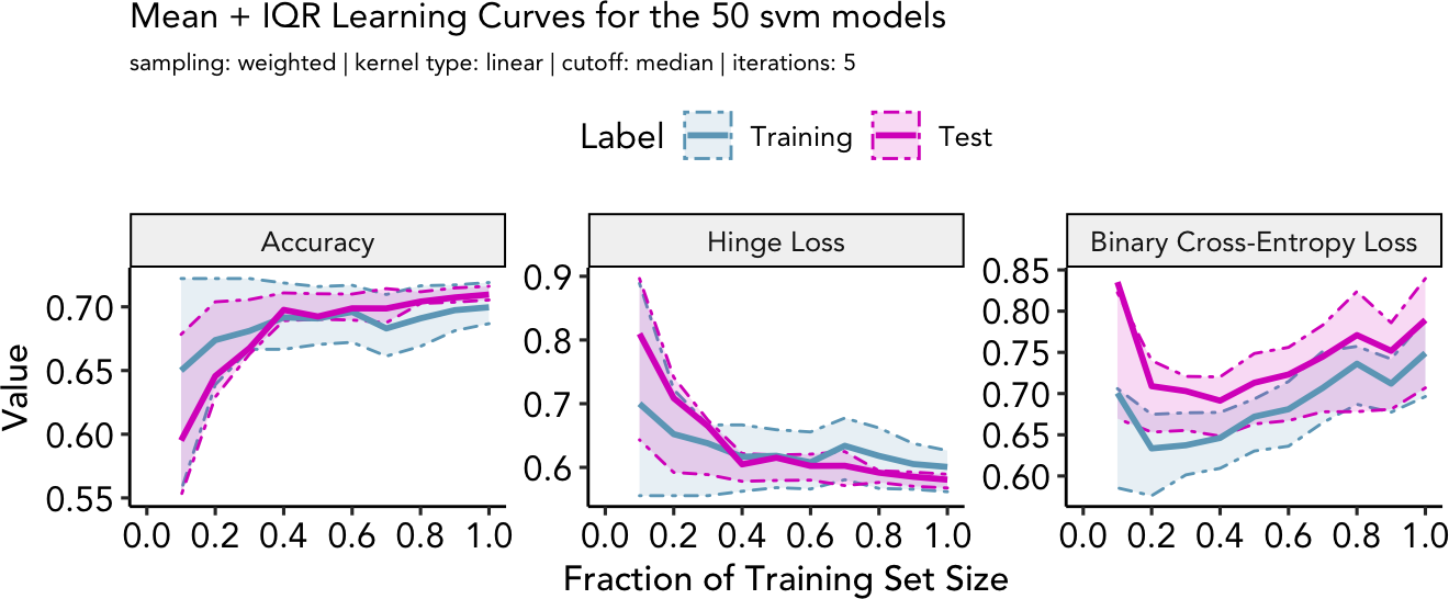
- Accuracy, (B) Hinge Loss, (C) Binary Cross-Entropy Loss
Appendix
Session info
#> R version 4.2.1 (2022-06-23)
#> Platform: x86_64-apple-darwin17.0 (64-bit)
#> Running under: macOS Big Sur ... 10.16
#>
#> Matrix products: default
#> BLAS:   /Library/Frameworks/R.framework/Versions/4.2/Resources/lib/libRblas.0.dylib
#> LAPACK: /Library/Frameworks/R.framework/Versions/4.2/Resources/lib/libRlapack.dylib
#>
#> locale:
#> [1] en_US.UTF-8/en_US.UTF-8/en_US.UTF-8/C/en_US.UTF-8/en_US.UTF-8
#>
#> attached base packages:
#> [1] stats     graphics  grDevices utils     datasets  methods   base
#>
#> other attached packages:
#>  [1] binaryPPIclassifier_1.5.5.8 plotly_4.10.0
#>  [3] varhandle_2.0.5             usethis_2.1.6
#>  [5] tidyr_1.2.0                 tibble_3.2.1
#>  [7] stringr_1.4.1               Rmisc_1.5.1
#>  [9] plyr_1.8.7                  rlang_1.1.1
#> [11] randomForest_4.7-1.1        purrr_1.0.1
#> [13] plotROC_2.3.0               ggnewscale_0.4.7
#> [15] e1071_1.7-11                DescTools_0.99.46
#> [17] cowplot_1.1.1               caret_6.0-94
#> [19] lattice_0.20-45             viridis_0.6.2
#> [21] viridisLite_0.4.1           ggpubr_0.4.0
#> [23] ggplot2_3.3.6               dplyr_1.1.2
#> [25] BiocStyle_2.24.0
#>
#> loaded via a namespace (and not attached):
#>   [1] colorspace_2.0-3     ggsignif_0.6.3       class_7.3-20
#>   [4] rprojroot_2.0.3      fs_1.5.2             gld_2.6.5
#>   [7] rstudioapi_0.14      proxy_0.4-27         farver_2.1.1
#>  [10] listenv_0.8.0        prodlim_2023.03.31   fansi_1.0.3
#>  [13] mvtnorm_1.1-3        lubridate_1.8.0      codetools_0.2-18
#>  [16] splines_4.2.1        cachem_1.0.6         rootSolve_1.8.2.3
#>  [19] knitr_1.40           jsonlite_1.8.0       pROC_1.18.2
#>  [22] broom_1.0.1          httr_1.4.4           BiocManager_1.30.18
#>  [25] compiler_4.2.1       backports_1.4.1      assertthat_0.2.1
#>  [28] lazyeval_0.2.2       Matrix_1.4-1         fastmap_1.1.0
#>  [31] cli_3.6.1            htmltools_0.5.3      tools_4.2.1
#>  [34] gtable_0.3.1         glue_1.6.2           lmom_2.9
#>  [37] reshape2_1.4.4       Rcpp_1.0.9           carData_3.0-5
#>  [40] cellranger_1.1.0     jquerylib_0.1.4      pkgdown_2.0.6
#>  [43] vctrs_0.6.3          nlme_3.1-159         iterators_1.0.14
#>  [46] timeDate_4022.108    gower_1.0.1          xfun_0.32
#>  [49] globals_0.16.1       lifecycle_1.0.3      rstatix_0.7.0
#>  [52] future_1.27.0        MASS_7.3-58.1        scales_1.2.1
#>  [55] ipred_0.9-14         ragg_1.2.2           parallel_4.2.1
#>  [58] expm_0.999-6         yaml_2.3.5           Exact_3.2
#>  [61] memoise_2.0.1        gridExtra_2.3        sass_0.4.2
#>  [64] rpart_4.1.16         stringi_1.7.8        highr_0.9
#>  [67] desc_1.4.1           foreach_1.5.2        hardhat_1.3.0
#>  [70] boot_1.3-28          lava_1.7.2.1         pkgconfig_2.0.3
#>  [73] systemfonts_1.0.4    evaluate_0.16        labeling_0.4.2
#>  [76] htmlwidgets_1.5.4    recipes_1.0.6        tidyselect_1.2.0
#>  [79] parallelly_1.32.1    magrittr_2.0.3       bookdown_0.28
#>  [82] R6_2.5.1             generics_0.1.3       pillar_1.9.0
#>  [85] withr_2.5.0          survival_3.4-0       abind_1.4-5
#>  [88] nnet_7.3-17          future.apply_1.9.0   car_3.1-0
#>  [91] utf8_1.2.2           rmarkdown_2.16       grid_4.2.1
#>  [94] readxl_1.4.1         data.table_1.14.2    ModelMetrics_1.2.2.2
#>  [97] digest_0.6.29        textshaping_0.3.6    stats4_4.2.1
#> [100] munsell_0.5.0        bslib_0.4.0